This article will show how Magcam inspects a radial flux permanent magnet rotor from a servo motor.
Specifically, multiple analysis methods for detecting magnetic issues with the rotor will be presented. These methods are included in MagScope, Magcam’s in-house developed software. The magnetic data can be obtained with either Magcam’s Rotor Scanner or Magcam’s Combi Scanner for flat magnets and rotor assemblies.
The analyses in this article include the following:
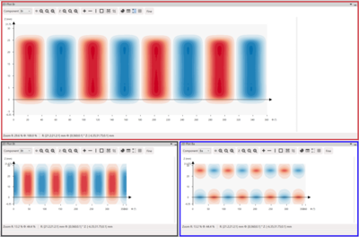
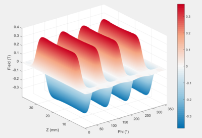
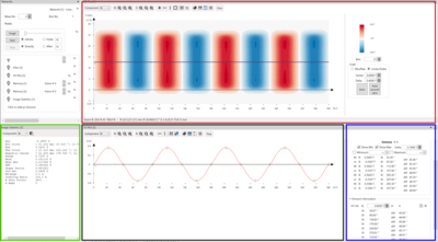
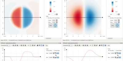
- Magnetic field plot analysis
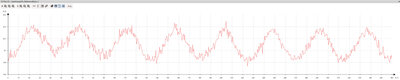
- Pole analysis (1D cutout analysis)
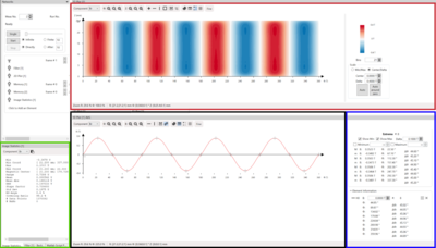
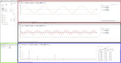
- Average 1D analysis
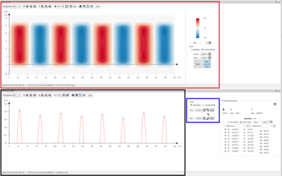
- Average peak variations
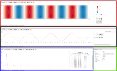
- Fourier analysis
- Cogging torque analysis
Let’s dive right in.
Before the magnetic measurement, a laser measurement is performed to define the rotor’s angular position and to be able to correct for runout.